I wrote this in April 2017, when Kaggle datasets were the easiest way to practise on something that looked like real business data. The Human Resources Analytics dataset was popular that year. It had a clean binary outcome (did the employee leave or not) and a handful of traits that anyone could reason about.
What I wanted was a quick way to answer one question: which combinations of employee characteristics carry the highest turnover? In 2017 I wrote a 130-line R function for it and read the results off the RStudio viewer. For this revision I re-ran the whole investigation in Python on the same data, kept the questions in their original order, and then went two steps further than I could in 2017: a picture of who actually leaves, and a model that weighs every trait at once. One of my 2017 conclusions did not survive the re-run. I have left it in and said so.
Simple risk segmenting
I call this simple risk segmenting. You take a population, split it by one or two characteristics, and look at the share of each group that had the bad outcome. In this case the bad outcome is leaving the company, and I call the share in each group the turnover rate.
The output is a matrix. Rows are the groups of the first characteristic, columns are the groups of the second, and each cell is the probability of turnover for employees who fall into both. It is a conditional probability table, nothing more. Its value is that it is fast to build and easy to show to someone who does not care about models.
The data
The dataset has 14,999 employees and one row each. The outcome column left is 1 for the 3,571 people who left, so the company-wide turnover rate is 23.8%. The other nine columns are the traits.
| Column | Meaning |
|---|---|
satisfaction_level | Employee satisfaction on a 0 to 1 scale |
last_evaluation | Score on the employee’s last evaluation |
number_project | Number of projects the employee has worked on |
average_monthly_hours | Average hours worked per month |
time_spent_company | Years at the company |
work_accident | 1 if the employee had a workplace accident |
promotion_last_5years | 1 if promoted in the last five years |
department | The employee’s department (called sales in the 2017 file) |
salary | Salary band: low, medium or high |
The copy of the file I used this time has the column typos fixed, so average_montly_hours is now spelled properly. Nothing else changed.
The rate function
In 2017 the function was most of the post. It grouped each characteristic by hand, counted leavers and stayers with nested which() calls, and glued the result into a matrix. In pandas the same job is a pivot table.
import pandas as pd

hr = pd.read_csv("HR_comma_sep.csv")


def rate_matrix(df, y, c1, c2=None, bins=20):
    """Turnover rate for every combination of two traits.

    Continuous columns are cut into equal-width ranges; integer and
    text columns keep one group per value.
    """
    def group(col):
        s = df[col]
        if s.dtype.kind == "f":
            return pd.cut(s, bins=bins)
        return s

    if c2 is None:
        return df.groupby(group(c1), observed=True)[y].mean()
    return df.pivot_table(index=group(c1), columns=group(c2),
                          values=y, aggfunc="mean", observed=True)
Because left is 0 or 1, the mean of a group is its turnover rate. The rest of the post is this function called five times, with a seaborn heatmap on the result.
The investigation
Are employees with low satisfaction more likely to leave?
by_satisfaction = rate_matrix(hr, "left", "satisfaction_level")
I used 20 ranges for no deeper reason than wanting enough detail to see a pattern. The result confirmed the obvious part and raised a less obvious one.
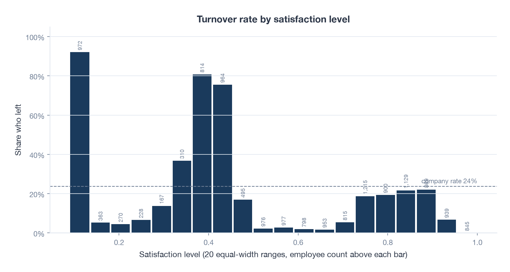
| Satisfaction range | Employees | Turnover rate |
|---|---|---|
| 0.09 to 0.14 | 972 | 92% |
| 0.36 to 0.41 | 814 | 81% |
| 0.41 to 0.45 | 964 | 75% |
| 0.73 to 0.91 | 4,113 | 19% to 22% |
| 0.95 to 1.00 | 845 | 0% |
The least satisfied employees almost all leave and the most satisfied never do. That is the obvious part. The surprise is the band just below the middle. Employees scoring 0.36 to 0.45 left at 75% to 81%, far above their neighbours on either side, and there are 1,778 of them. Mildly unhappy people were leaving at a rate that stood out. That was the part worth chasing.
Does the pattern hold across job functions?
My first guess was that the odd band was tied to one department.
by_department = rate_matrix(hr, "left", "satisfaction_level", "department")
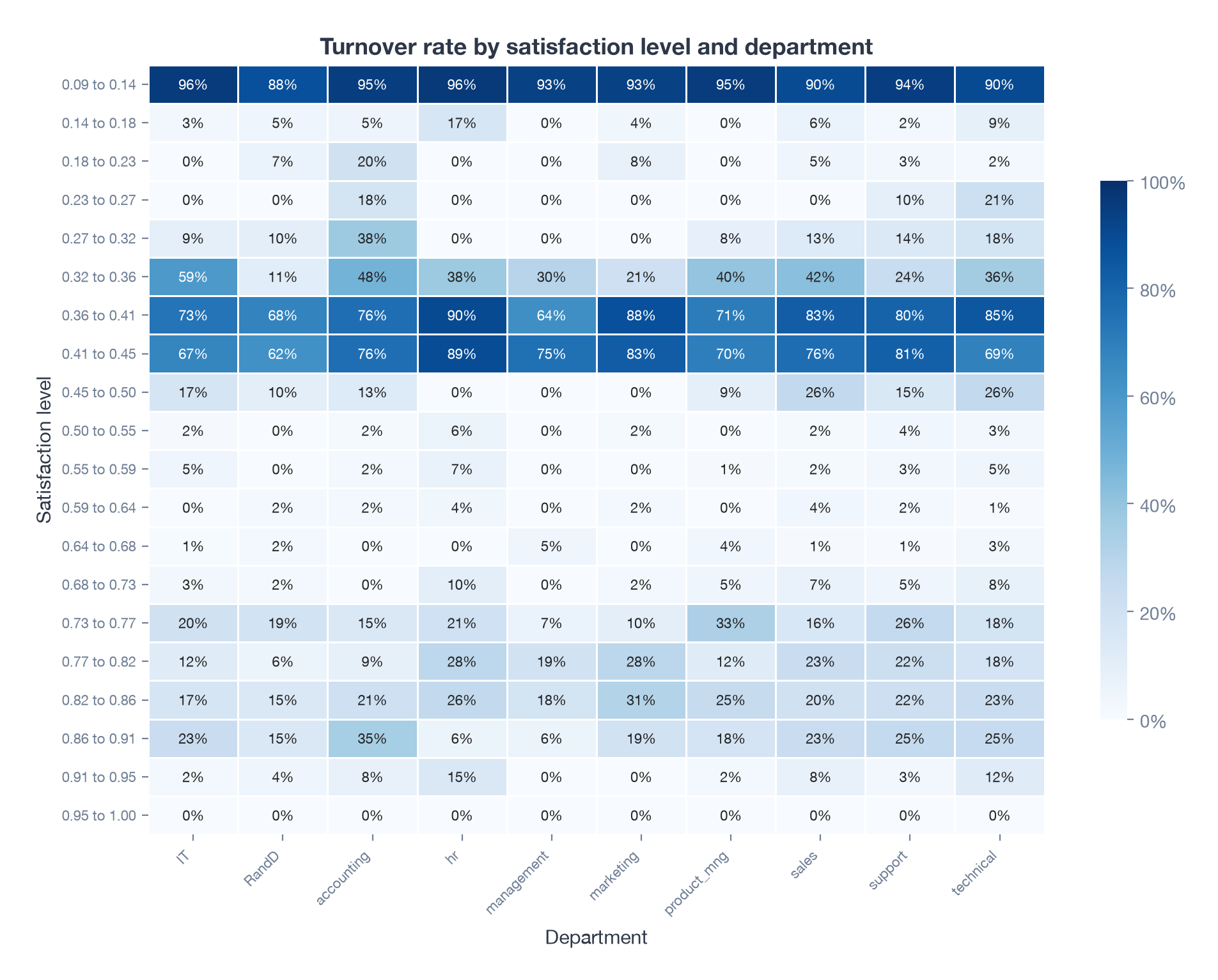
It held everywhere. The 0.36 to 0.45 band runs at 62% to 90% in every department, from R&D at the low end to HR at the high end. Department on its own barely matters: management has the lowest overall rate at 14% and HR the highest at 29%, and everything else sits between 22% and 27%. Whatever was going on, somewhat unhappy workers were leaving regardless of the kind of work they did.
Is it about hours worked?
Next I thought these employees might be overworked. Crossing satisfaction with monthly hours, cut into ranges of 20 hours, would show it.
hr["hours_range"] = pd.cut(hr["average_monthly_hours"], bins=range(80, 330, 20))
by_hours = hr.pivot_table(index=pd.cut(hr["satisfaction_level"], 20),
                          columns="hours_range", values="left",
                          aggfunc="mean", observed=True)
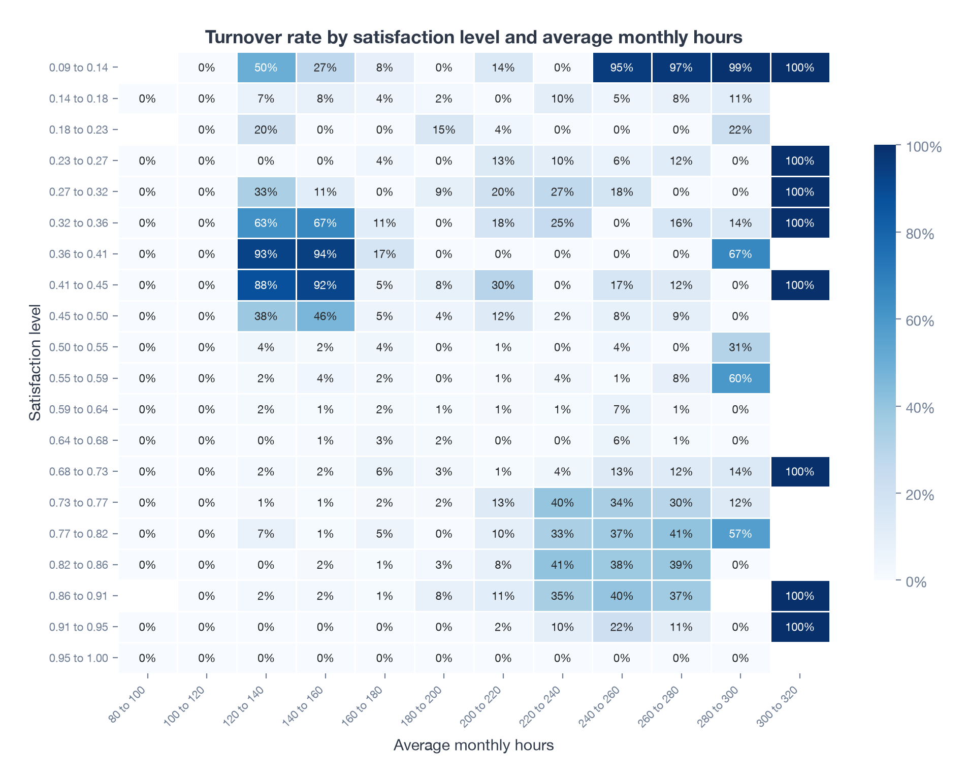
The band’s turnover is concentrated in two cells: 93% at 120 to 140 hours a month and 94% at 140 to 160. Move to 160 to 180 hours and the same satisfaction band drops to 17%, then to zero.
That surprised me in 2017 and still does. A full-time employee works at least 160 hours a month (40 hours a week, four weeks). The risk was highest for people working less than a full-time schedule, the opposite of my overwork theory. Leavers in the band worked a median of 145 hours a month; the stayers in the same band worked 169. My conclusion at the time was that the highest-risk group was likely contract, seasonal or part-time staff.
The heatmap also shows the overwork story I had expected, just in a different corner. The least satisfied employees who work 240 hours or more leave at 95% to 100%. Those are two different groups of leavers, and a one-way cut on satisfaction had lumped them together.
Does project count support that?
If these are short-term or part-time workers, they should also have fewer projects.
by_projects = rate_matrix(hr, "left", "satisfaction_level", "number_project")
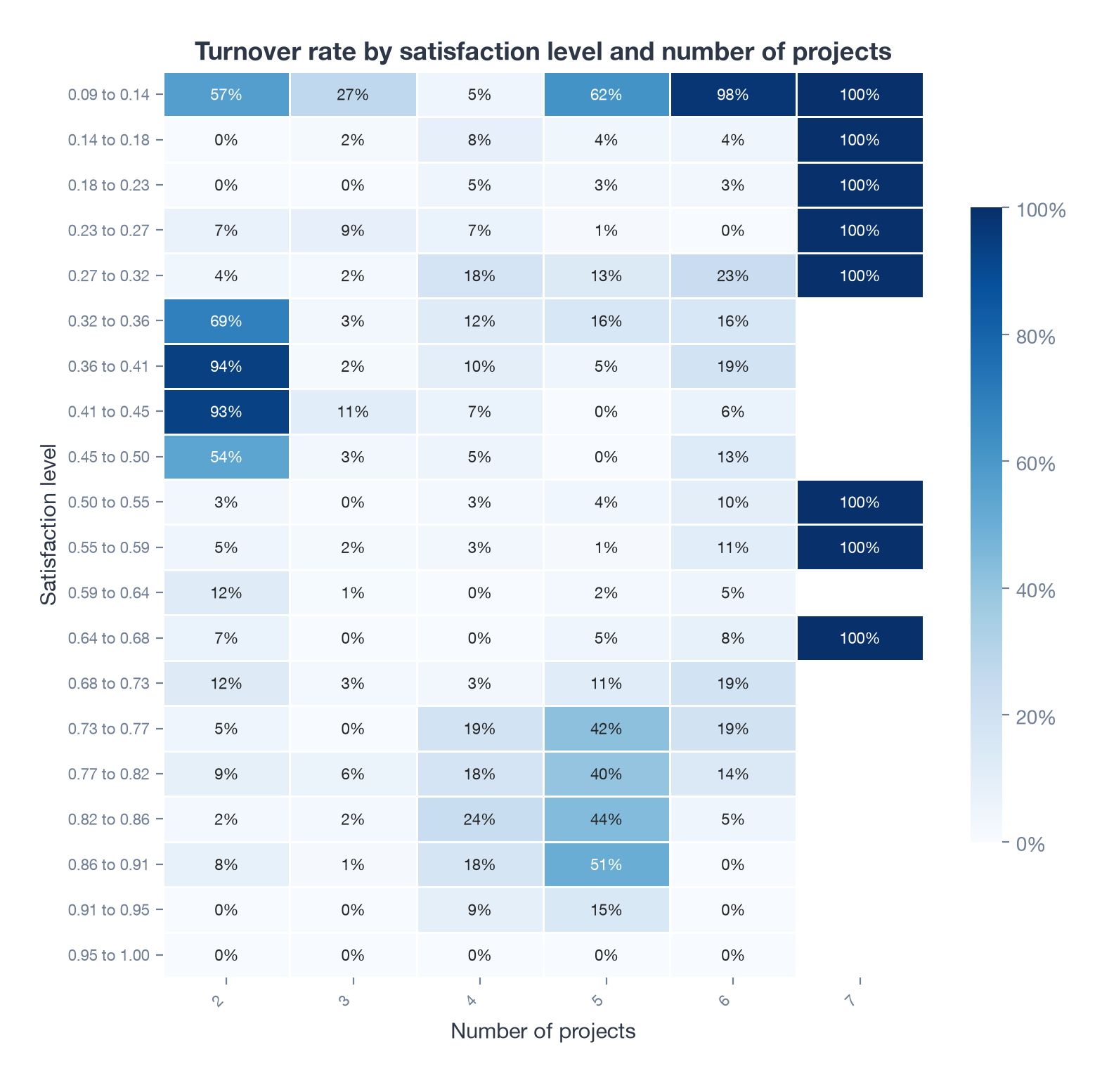
They do. In the 0.36 to 0.45 band, employees with exactly two projects leave at 93%, and there are 1,530 of them. With three or more projects the rate collapses to between 2% and 19%. That fits the picture of people who join, do a little work, and go.
The other corner shows up again too. Among the least satisfied, six or seven projects means a 98% to 100% exit rate. Too little work and too much work both end the same way, for different kinds of employee.
Does a workplace accident make it worse?
The last question in 2017 was whether these employees were having a hard time on the job itself. I filtered to employees who had a workplace accident and re-ran the satisfaction by projects matrix.
accident = hr[hr["work_accident"] == 1]
by_projects_accident = rate_matrix(accident, "left", "satisfaction_level", "number_project")
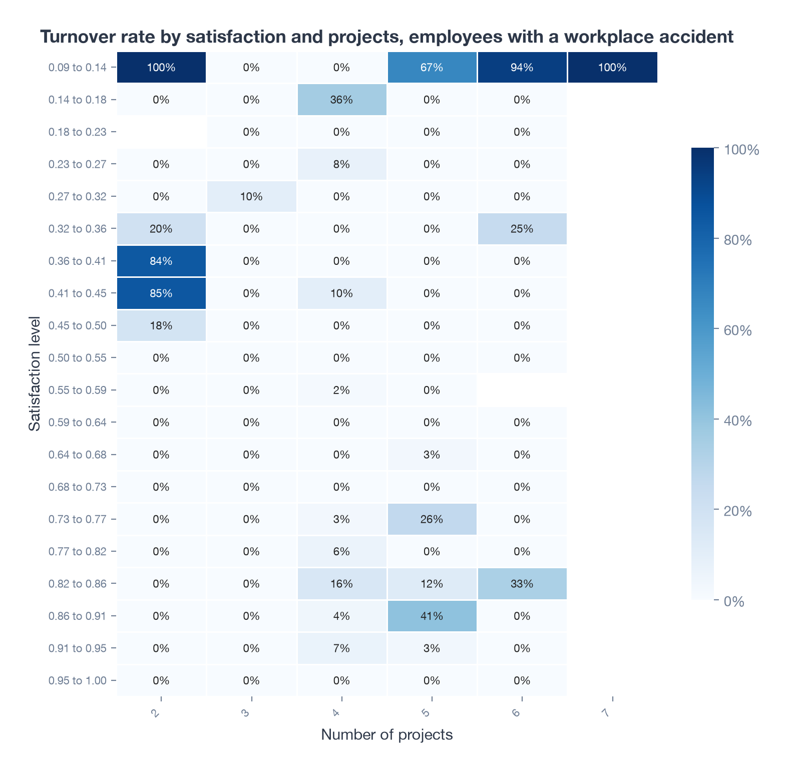
In 2017 I read the result as “accidents add to the risk for this group”. The re-run says the opposite. Inside the 0.36 to 0.45 band, employees with an accident on record left at 50%, against 78% for the band as a whole. Across the whole company, people with an accident left at 7.8% and people without at 26.5%.
That does not mean accidents keep people at a company. The likelier reading is survivorship: the longer you have been somewhere, the more chance you have had of an accident being recorded, and long-tenured people are the ones who stay. In 2017 I was comparing cells by eye across two separate matrices and I saw what I was looking for. Putting the numbers side by side would have caught it.
What I concluded in 2017
The highest-risk employees were not the overworked ones I set out to find. They were mildly unhappy, under-used people on two projects and short hours, most likely contract or part-time staff, and the pattern held in every department. That conclusion still holds. The extra claim about accidents does not.
The view I could not draw in 2017
A matrix answers the question you ask it. A scatter plot of every employee, satisfaction against hours, answers a question I had not thought to ask: how many distinct kinds of leaver are there?
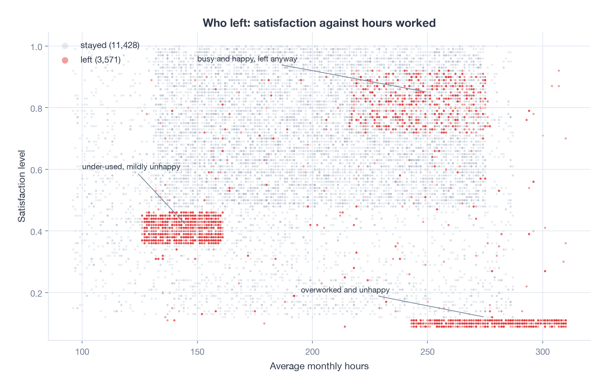
Three. Of the 3,571 people who left:
| Group | Leavers | Who they are |
|---|---|---|
| Under-used and mildly unhappy | 1,524 | Satisfaction 0.35 to 0.47, 125 to 165 hours a month, 99.5% on two projects |
| Overworked and unhappy | 882 | Satisfaction below 0.12, 240 hours a month or more, a median of six projects |
| Busy and happy | 888 | Satisfaction above 0.7, more than 210 hours a month |
The first group is the one the matrices found. The second is the overwork story. The third I had no theory for in 2017 and still find the most interesting: people who were satisfied, worked long hours and left anyway. In a real company that is the group you would want to interview, because they look like the people who got a better offer.
The tight rectangles in that plot are also a warning. Real HR data is never this clean. This dataset is widely believed to be simulated, and the sharp edges on every cluster support that. The method transfers; the exact numbers do not.
Letting a model weigh everything at once
A two-way matrix can only hold two traits. To see all nine together I fitted a gradient boosted classifier and asked SHAP which traits moved each prediction.
import lightgbm as lgb
import shap
from sklearn.model_selection import train_test_split

X = hr.drop(columns="left")
X["department"] = X["department"].astype("category")
X["salary"] = pd.Categorical(X["salary"], ["low", "medium", "high"], ordered=True)
y = hr["left"]

X_tr, X_te, y_tr, y_te = train_test_split(X, y, test_size=0.25,
                                          stratify=y, random_state=2017)
model = lgb.LGBMClassifier(n_estimators=400, learning_rate=0.03,
                           num_leaves=15, min_child_samples=40)
model.fit(X_tr, y_tr)

shap_values = shap.TreeExplainer(model).shap_values(X_te)
shap.summary_plot(shap_values, X_te)
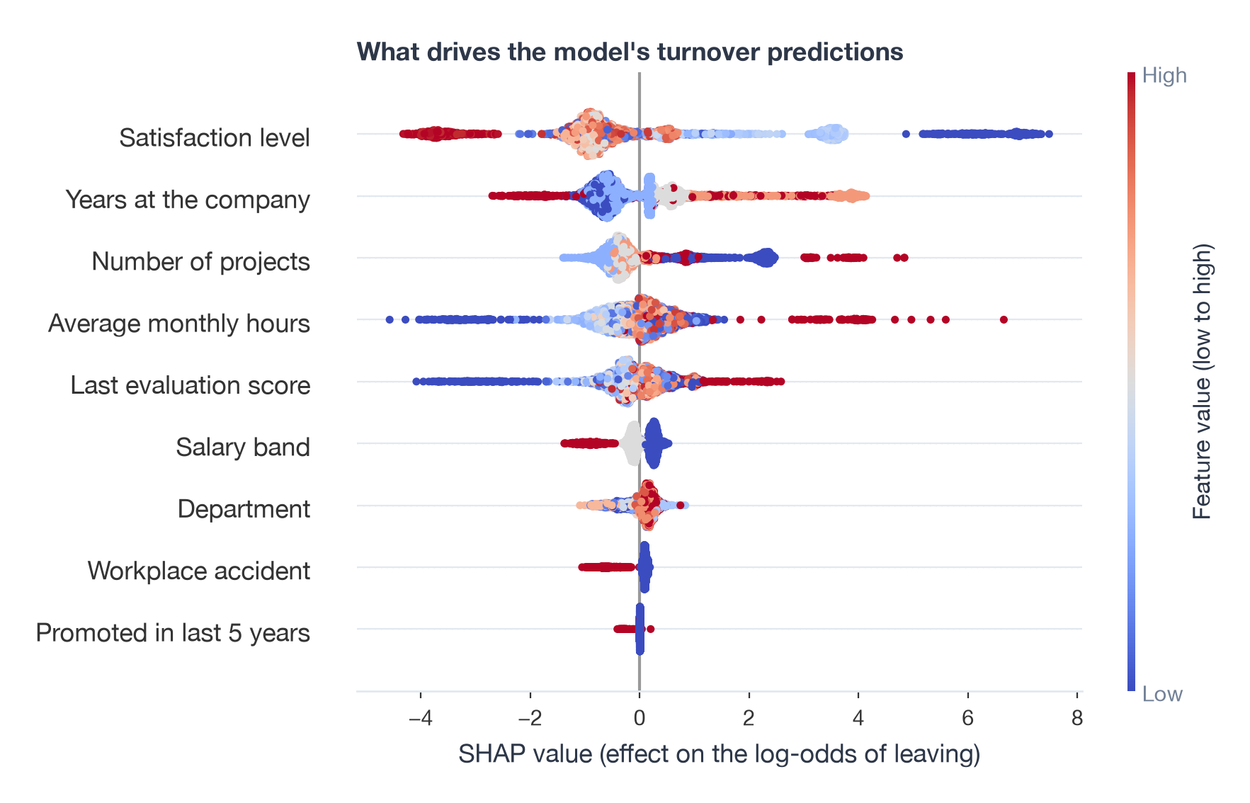
The model scores an AUC of 0.995 on the held-out quarter, which is another sign the data is simulated. The ranking is more useful than the score. Satisfaction matters most by a wide margin, then years at the company, number of projects, monthly hours and the last evaluation score. Salary band and department are minor. A promotion in the last five years hardly registers, mostly because so few people had one.
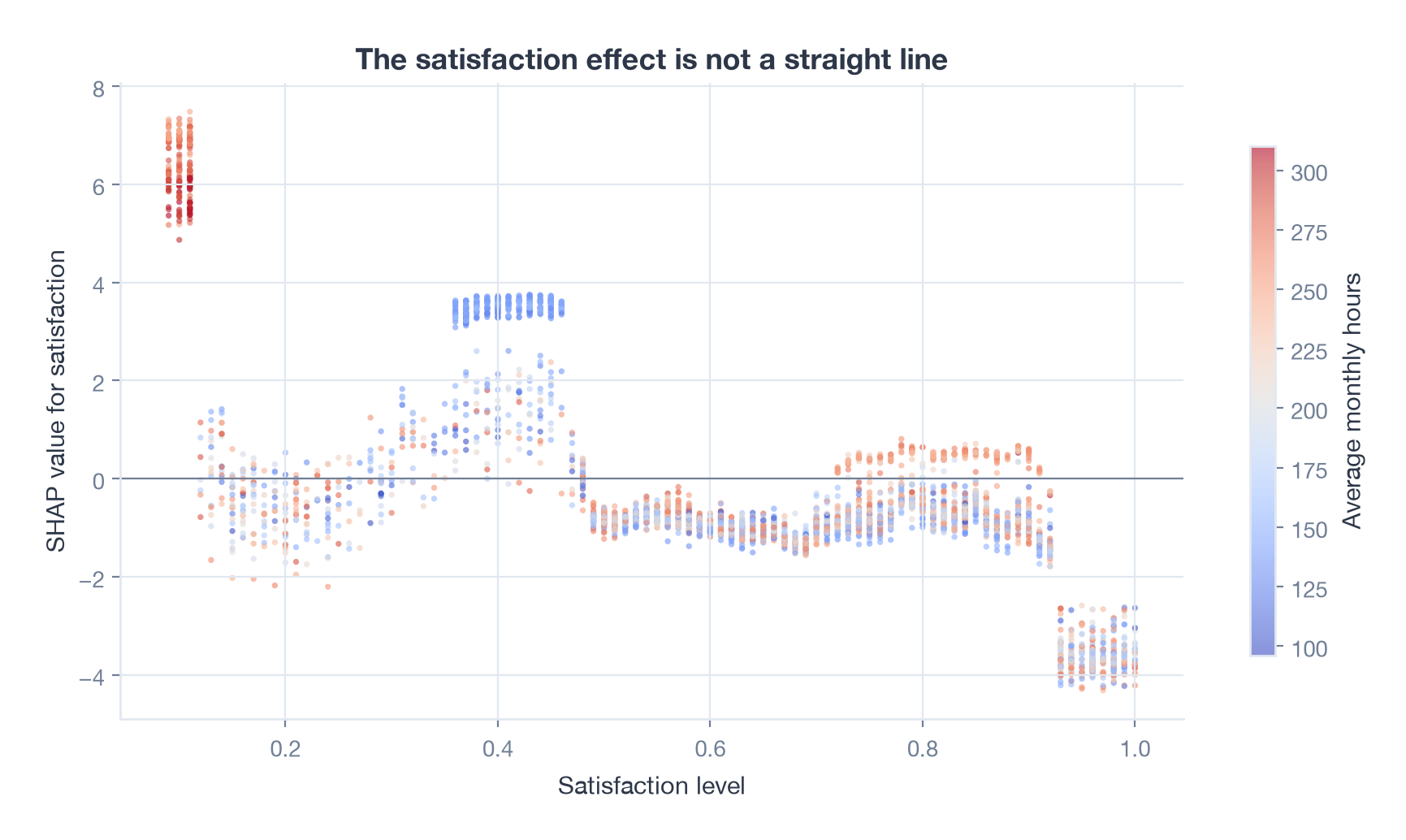
The dependence plot is the matrix investigation in one picture. The satisfaction effect is not a straight line. It spikes at the very bottom, drops to nothing, spikes again at 0.36 to 0.46 (the blue, low-hours points), goes quiet through the middle, and rises a little again around 0.75 to 0.9 for the high-hours employees. Each spike is one of the three clusters.
Looking back from 2026
The matrix method held up. It took me most of a day in 2017 and takes a few lines of pandas now, and it is still the right first move when someone asks “who is leaving?”, because a heatmap of rates needs no explanation in a meeting.
What the re-run taught me is to check the comparison, not just the cell. The accident claim was wrong because I compared one filtered matrix against my memory of another. Two numbers next to each other, 50% against 78%, settle it instantly. I would now put the counts in every cell as well as the rates, since a 100% cell with three people in it is noise.
A model earns its place after the matrices, not instead of them. SHAP gave me the same three groups the scatter plot shows, plus a ranking of everything else, and it did so without me choosing which pairs to cross. The cost is that a boosted model with an AUC of 0.995 tells you more about the dataset than about employees. On real data I would expect something closer to 0.75, and I would trust the matrices more than the model until the model had been through a year of out-of-time checks.
Two things this analysis still cannot do. It cannot say when someone will leave, which is what a survival model (Kaplan-Meier curves, a Cox model, or a boosted survival model) is for, and it would make the time-in-company effect much clearer than a cross-section does. And it cannot say what would change their mind, which is a causal question. An uplift model on a retention programme answers that, but only if the programme was rolled out as an experiment. A probability matrix shows who leaves. It never shows why.