I wrote this in 2018, when part of my job as a data scientist was to build, update and maintain a scorecard for small and medium business loans. A scorecard is a model that tells a lender which applicants are likely to pay back their loan and which are not. I could not share the data I worked with, so I rebuilt the whole process on public Lending Club data and published it as a five-part series in R.
This version is a full re-run, not an edit. I kept the 2018 structure, Lending Club’s 2015 loan book, and the method lenders still use (Weight of Evidence, Information Value, logistic regression, reject inference, a points-based score), and rebuilt it in Python with the habits I have picked up since. The honest result is a much weaker model than I reported in 2018, and the reasons why are the most useful part of the post. The short summary and the original R code live on the project page; the Python pipeline is in the same repository.
Why scorecards
Lenders have used scorecards for decades because they are easy to read, easy to audit and easy to put into a decision system. Every applicant gets a number. A higher number means lower risk. A credit officer can see which features pushed the number up or down, and a regulator can ask why a given applicant was declined and get a straight answer.
The method is the classic one in consumer and commercial lending:
- Collect, clean and label the data.
- Transform every feature with Weight of Evidence (WOE) and rank them with Information Value (IV).
- Train and validate a logistic regression on the WOE values.
- Check the scorecard on loans it has never seen, and correct for the applicants the lender never funded.
- Finish it with a grading scheme and a score.
Each section below follows one of those steps, and says what changed since 2018.
The Lending Club data
Lending Club was a peer-to-peer lender that published its loan book as CSV files, and still serves the 2015 files from its own site. LoanStats3d.csv holds every loan issued in 2015 with its final outcome; RejectStatsD.csv holds every application it turned down that year.
import pandas as pd

loans = pd.read_csv("LoanStats3d.csv", skiprows=1, low_memory=False)
loans = loans[loans["id"].notna()]                     # trailing summary lines
loans = loans[loans["term"].str.strip() == "36 months"]
loans["bad"] = (loans["loan_status"] == "Charged Off").astype(int)
| Step | Loans |
|---|---|
| In the 2015 file | 421,095 |
| 36-month term | 283,173 |
| Fully Paid (good) | 240,995 |
| Charged Off (bad) | 42,178 |
The bad rate is 14.9%. In 2018 some loans were still open, so I had to drop the ones without a final status. Every 2015 loan has now run its course, which makes the labels cleaner than they were.
Features: only what a lender knows at application time
This is the first place the re-run differs, and it is the one that matters most. A scorecard is used at the moment of application, so it may only use what is known at that moment. The 2015 file has 150 columns, and a lot of them describe what happened to the loan afterwards: payments received, recoveries on charged-off loans, the date of the last payment, the collection fee. Any of those will make a model look brilliant on paper and useless in production, because they are the outcome wearing a disguise.
I also left out Lending Club’s own pricing. The grade, sub-grade, interest rate and installment are outputs of Lending Club’s scorecard. Using them would score their model, not the applicant.
EXCLUDED = {
    "pricing": ["int_rate", "grade", "sub_grade", "installment"],
    "post_origination": ["funded_amnt", "out_prncp", "total_pymnt", "total_rec_prncp",
                         "total_rec_int", "total_rec_late_fee", "recoveries",
                         "collection_recovery_fee", "last_pymnt_d", "last_pymnt_amnt",
                         "next_pymnt_d", "last_credit_pull_d", "hardship_*", "settlement_*"],
    "identifiers_free_text": ["id", "member_id", "url", "desc", "title", "emp_title"],
    "fairness_proxy": ["zip_code"],
}
Zip code is out for a different reason. At three-digit grain it is a proxy for race, which fair lending rules do not allow a lender to use. State stays in as a coarse regional term; in production it would get the same review.
That left 62 candidate features: loan amount, income, debt-to-income ratio, home ownership, purpose, employment length, and the credit bureau attributes (inquiries, open accounts, balances, limits, months since the last delinquency, and so on). Two gaps against 2018: this export of the file no longer carries the FICO range, so there is no bureau score in the model, and the newer bureau fields Lending Club added in late 2015 are empty for the first nine months of the year, so they cannot be learned either.
Split by time, not at random
In 2018 I split the loans 75/25 at random. The 2026 habit is to split by issue date: train on loans issued January to September 2015, test on October to December. A random split lets the model learn from loans issued the same week as the ones it is tested on. An out-of-time split is closer to what happens when a scorecard goes live, which is that it scores applicants who arrive after every loan it was built on.
| Window | Loans | Bad rate |
|---|---|---|
| Train, January to September 2015 | 194,363 | 14.9% |
| Test, October to December 2015 | 88,810 | 14.8% |
The bad rate was stable across 2015, between 14.1% and 15.7% by month, so the time split did not cost anything here. It usually does.
Information Value and Weight of Evidence
Weight of Evidence replaces each raw value with the log of the ratio of goods to bads in its bin, so every feature sits on the same log-odds scale a logistic regression works in. Information Value sums the WOE across the bins, weighted by how different the good and bad shares are, and gives one number per feature for how well it separates good from bad on its own. Siddiqi’s rule of thumb: under 0.02 is useless, 0.02 to 0.1 weak, 0.1 to 0.3 medium, above 0.5 suspicious.
In 2018 the binning came from R’s Information package with its default ten equal-frequency bins. Today optbinning finds the bins by solving a small optimisation that keeps the WOE trend monotonic where the data supports it, and handles categorical features and missing values in the same pass. It also takes the IV threshold as a selection rule, so the feature screen happens inside the fit.
from optbinning import BinningProcess

binning = BinningProcess(
    variable_names=FEATURES,
    categorical_variables=CATEGORICAL,
    selection_criteria={"iv": {"min": 0.02}},
    binning_fit_params={c: {"monotonic_trend": "auto_asc_desc"} for c in NUMERIC},
)
binning.fit(X_train, y_train)          # training window only

W_train = binning.transform(X_train, metric="woe")
W_test = binning.transform(X_test, metric="woe")
Bins are fitted on the training window only. In 2018 I binned the whole data set before splitting it, which leaks a little of the test set into the bins.
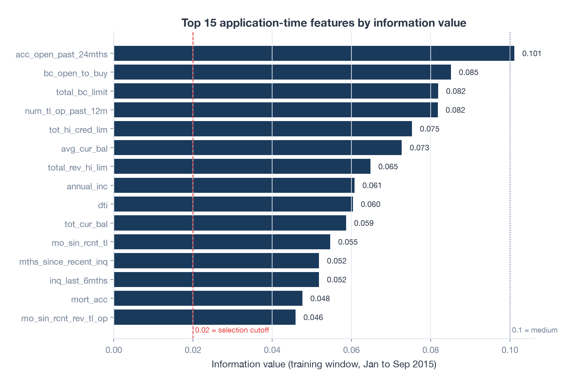
Of 62 candidates, 27 pass the 0.02 line. The strongest feature, the number of accounts opened in the past 24 months, has an IV of 0.10. Nothing reaches “medium”. That is what honest application-time features look like on unsecured consumer loans: every one is weak, and the model works by adding many weak signals together.
Reading WOE plots
The two features I singled out in 2018 are still worth looking at, for different reasons.
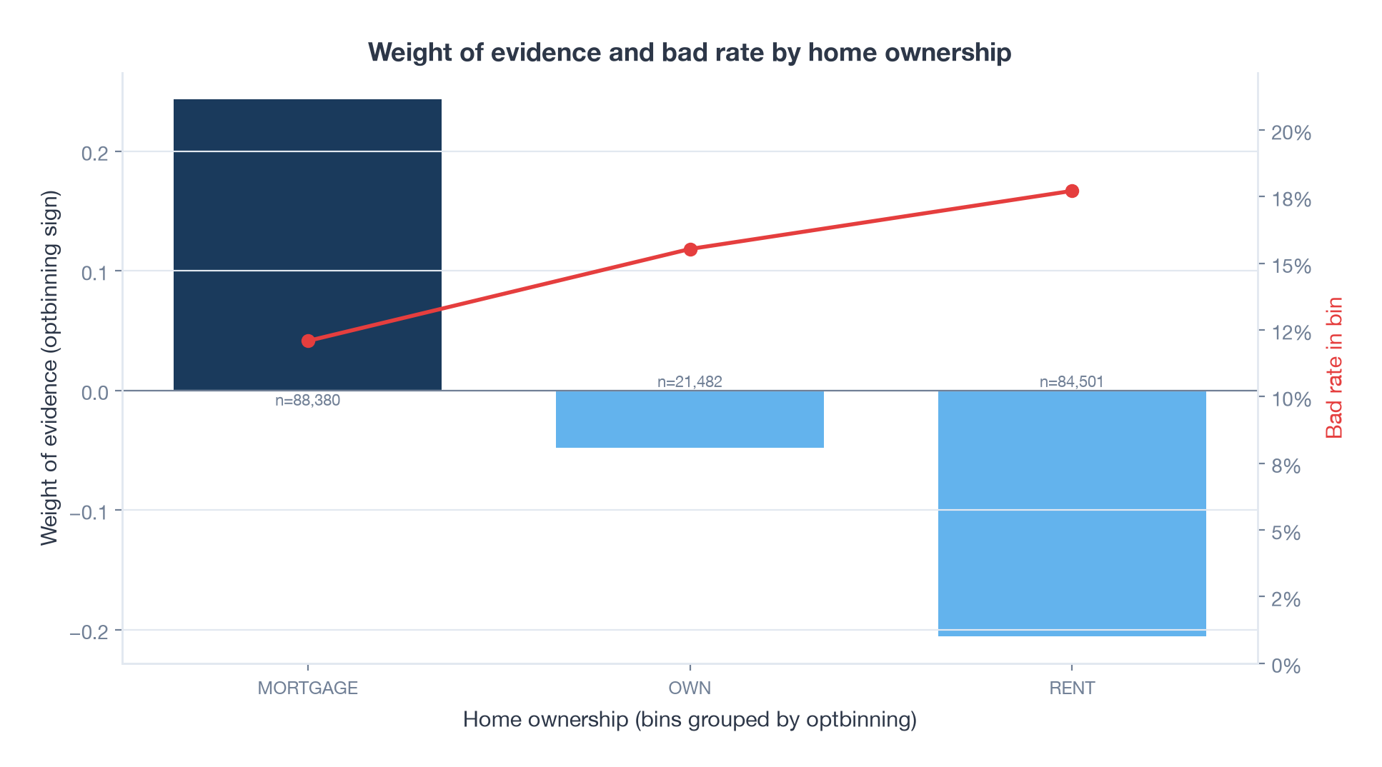
Home ownership. The 2018 reading holds. Borrowers paying a mortgage default at 12.1%, owners at 15.5%, renters at 17.7%. The WOE for mortgage is 0.24, against 0.29 in 2018, so the signal is stable across the two data cuts.
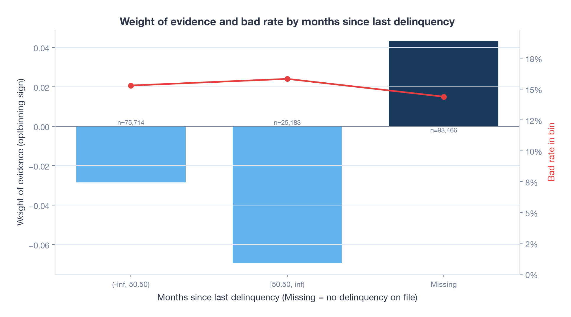
Months since last delinquency. In 2018 I made a story out of this feature: the longer since a delinquency the better, with an odd dip at 19 to 31 months that I put down to reporting lag. On the 2015 book it is nearly useless. The IV is 0.002. Borrowers with no delinquency on file default at 14.4%, and the two bins with one default at 15.3% and 15.8%. The 2018 story was a story about ten equal-frequency bins on a noisy feature, which is the kind of pattern that goes away when the binning is allowed to merge bins that do not differ.
Logistic regression on WOE features
The model is the same as 2018: a logistic regression with an L1 penalty, which can push a feature’s coefficient to exactly zero and drop it from the scorecard. In 2018 that was caret tuning glmnet over alpha and lambda. Here it is scikit-learn tuning the inverse penalty C by five-fold cross-validation on ROC AUC.
from sklearn.linear_model import LogisticRegression
from sklearn.model_selection import GridSearchCV, StratifiedKFold

grid = GridSearchCV(
    LogisticRegression(l1_ratio=1.0, solver="liblinear", max_iter=2000),
    {"C": [1e-4, 3e-4, 1e-3, 3e-3, 1e-2, 3e-2, 1e-1, 1.0]},
    scoring="roc_auc", cv=StratifiedKFold(5, shuffle=True, random_state=2018),
)
grid.fit(W_train, y_train)
model = grid.best_estimator_
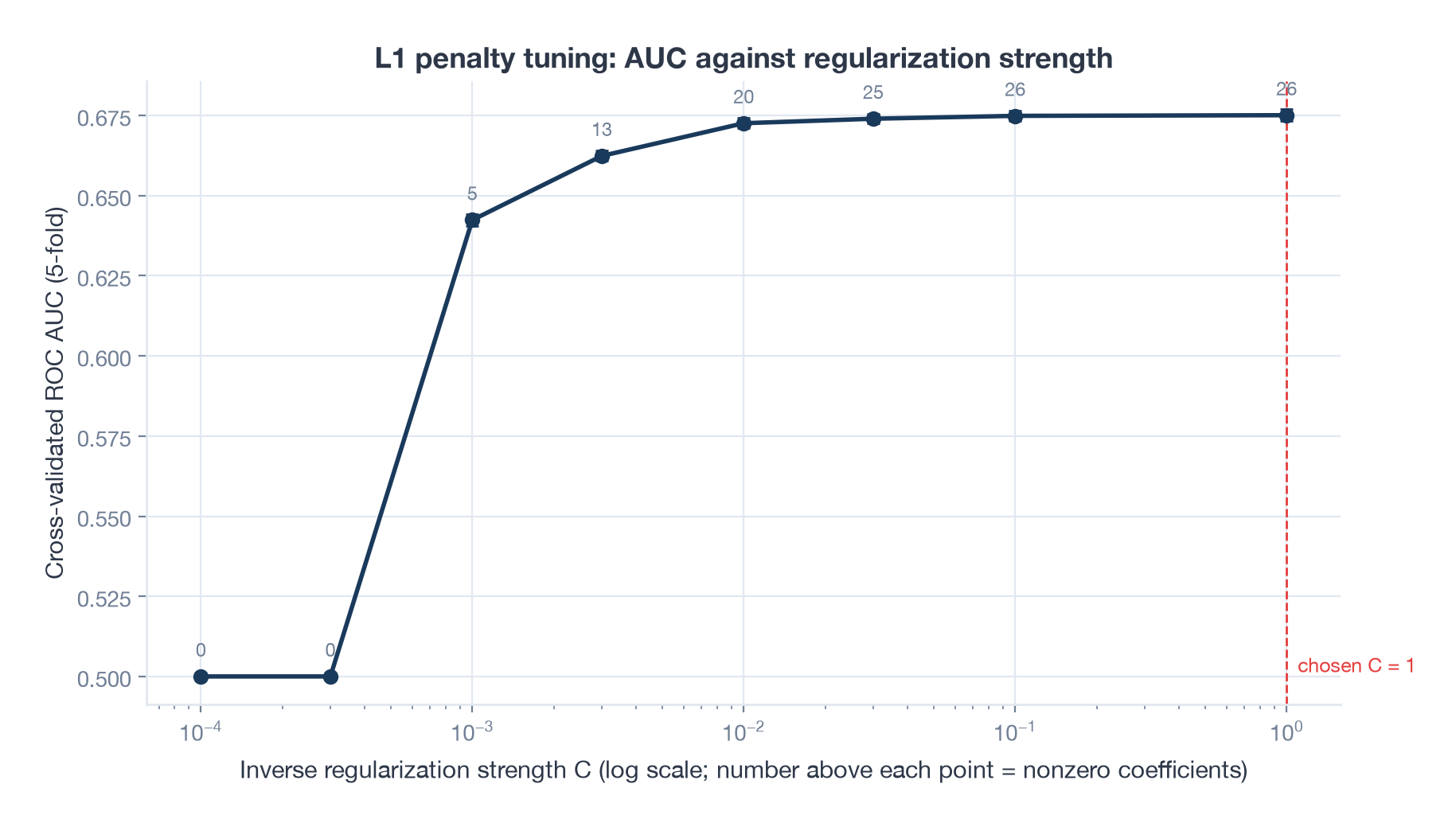
The AUC is flat from C = 0.03 upward, and the search picked the top of the grid. With 194,000 loans and 27 weak features, the penalty has very little to do. The L1 term zeroed exactly one feature.
One check I did not do in 2018: five of the surviving coefficients had the wrong sign. Total current balance, revolving balance, average balance, months since the most recent revolving account and length of credit history all came out saying that more was riskier, when their own WOE tables say the opposite. That is collinearity between the balance and limit features, and a scorecard cannot carry it, because the points for those features would run backwards. I dropped them one at a time, largest offender first, refitting each time. It cost 0.002 of AUC and left 21 features, all pointing the right way.
Validation
| Check | ROC AUC | Gini | KS |
|---|---|---|---|
| 5-fold cross-validation, training window | 0.674 | ||
| Random 75/25 split, for comparison with 2018 | 0.670 | ||
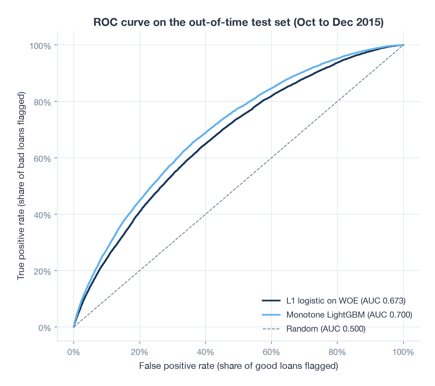
| Out-of-time test, October to December 2015 | 0.673 | 0.345 | 0.251 |
In 2018 I reported a cross-validated AUC of 0.8755 and a test AUC of 0.8792. The honest number on the same loan book is 0.67.
The gap is not the tooling. The 2018 feature list kept a few columns that only exist after the loan is issued, the collection recovery fee among them, and any one of them is enough to lift an AUC by 0.2. I did not notice because the 2018 test set was a random quarter of the same loans, which cannot catch leakage of that kind. Nothing in the method was wrong. The feature screen was.
An AUC of 0.67 on application-time data without a bureau score is ordinary for unsecured consumer lending. Lenders live in the 0.65 to 0.75 range on this kind of book, and the bureau score is usually what moves them toward the top of it.
A gradient boosted challenger
In 2018 I said I could have tried random forests and boosted trees and did not, because the goal was a scorecard. Today the standard move is to fit a boosted model as a challenger and see how much the scorecard leaves on the table. The trick that makes the challenger acceptable in a lending context is monotone constraints: each feature is forced to push risk in one direction, the direction of its WOE trend, so the model can be explained to a credit officer the same way a scorecard can.
import lightgbm as lgb

constraints = [monotone_sign(c) for c in FEATURES]   # +1, -1 or 0 from the WOE trend
challenger = lgb.LGBMClassifier(
    n_estimators=3000, learning_rate=0.03, num_leaves=31, min_child_samples=200,
    subsample=0.8, subsample_freq=1, colsample_bytree=0.7,
    monotone_constraints=constraints, monotone_constraints_method="basic",
)
challenger.fit(X_fit, y_fit, eval_set=[(X_val, y_val)], eval_metric="auc",
               callbacks=[lgb.early_stopping(100)])
| Model | Out-of-time AUC | Gini | KS |
|---|---|---|---|
| L1 logistic regression on WOE, 21 features | 0.673 | 0.345 | 0.251 |
| LightGBM, monotone constraints on 24 features | 0.700 | 0.400 | 0.293 |
| LightGBM, unconstrained | 0.703 | 0.405 | 0.296 |
The boosted model adds 0.027 of AUC. Keeping it monotone costs 0.002. That is the usual shape of the result: the trees find interactions the scorecard cannot, the gain is real but modest, and explainability is nearly free.
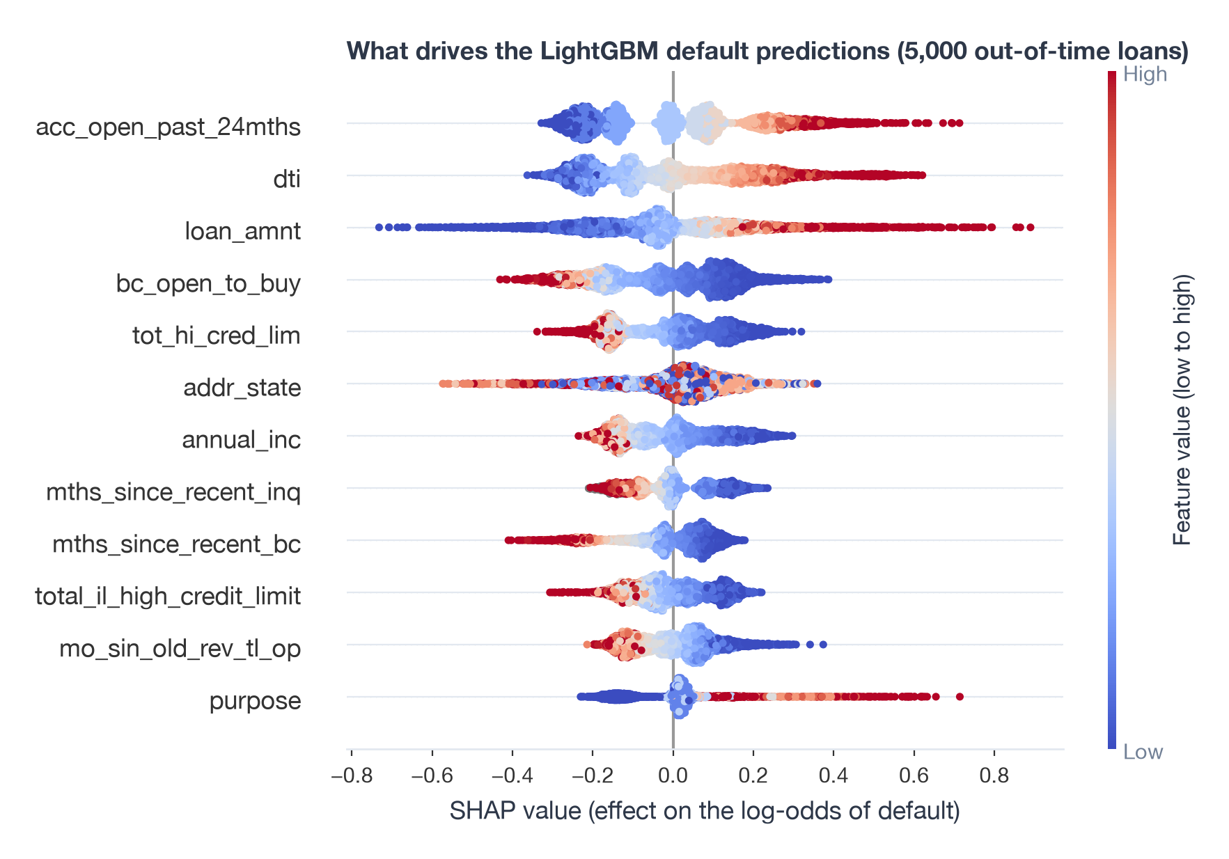
SHAP ranks the same features at the top as IV did, with one exception that is worth a sentence. Loan amount has an IV of 0.0001, so the univariate screen dropped it from the scorecard, yet it is third in the SHAP ranking. On its own the amount says nothing about risk. Together with income and credit limits it says a lot. A single-variable IV cannot see that, and it is the clearest argument for running a challenger even when you intend to ship the scorecard.
Reject inference with the real rejected applications
A scorecard is trained on funded loans, but it will be used on everyone who applies. The applicants the lender turned down have no outcome, and leaving them out biases the model toward the population that passed the old policy. Reject inference tries to put them back.
In 2018 I did this step wrong in two ways. I trained a small model on three features, then called predict with data= instead of newdata=, so R quietly returned fitted values for the accepted loans and I plotted those as the “rejected” distribution. And I had no real rejects to begin with. This time the 2015 rejected applications file is in the pipeline: 2.86 million applications, of which 1.96 million fall in the training window. I sampled 300,000 of those.
The catch with rejects is that the lender recorded very little about them. The two files share only the amount requested, the debt-to-income ratio, employment length and state. So the shared-feature model is a small one, and the method is augmentation by parcelling: score the rejects with it, cut them into score deciles, and in each decile label rejects as bad at twice the bad rate of accepted loans in the same score range. The factor of two is the usual assumption that rejected applicants are riskier than accepted ones who look the same on paper. It is an assumption, and everything downstream rests on it.
shared = ["loan_amnt", "dti", "emp_length", "addr_state"]
p_rejects = shared_model.predict_proba(W_rejects)[:, 1]
rejects["decile"], edges = pd.qcut(p_rejects, 10, labels=False, retbins=True)

for d in range(10):
    in_decile = rejects["decile"] == d
    accepted_rate = y_train[(p_accepted >= edges[d]) & (p_accepted < edges[d + 1])].mean()
    inferred_rate = min(2.0 * accepted_rate, 1.0)
    n_bad = round(inferred_rate * in_decile.sum())
    rejects.loc[rng.choice(rejects.index[in_decile], n_bad, replace=False), "bad"] = 1
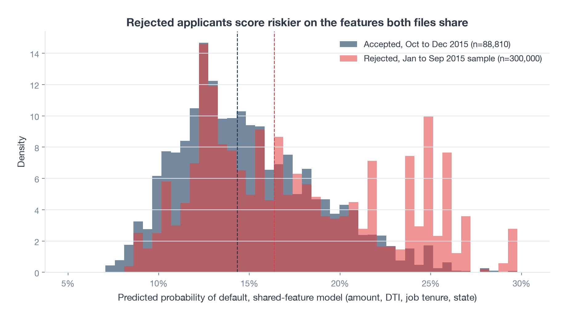
The rejects do score riskier, with a mean predicted default rate of 17.4% against 14.9% for accepted loans. The spikes on the right are the 21% of rejects with a debt-to-income ratio above 40, which no accepted loan has because it was Lending Club’s policy cap.
| Shared-feature model | Out-of-time AUC on real outcomes | IV of DTI | IV of employment length |
|---|---|---|---|
| Accepted loans only | 0.582 | 0.060 | 0.020 |
| Accepted plus inferred rejects | 0.574 | 0.196 | 0.189 |
The inferred labels make the IVs jump and make the model worse on real outcomes. Employment length is the tell: 89% of rejects have “less than 1 year” against 9% of accepted loans, which looks like a default value in the rejects file rather than a fact about applicants. Parcelling turns that artefact into a strong signal. This is the standard warning about reject inference. It mostly reflects the factor you chose and the fields you had, and it should never be judged on the augmented data, only on real outcomes.
Grade analysis
Lending Club sorted its loans into 25 sub-grades, A1 to G5. To mirror that, I cut the out-of-time test set into 25 equal-size bins by the scorecard’s predicted probability and looked at the observed bad rate in each. In 2018 I used equal-width bins, which left the top ones nearly empty; equal-frequency bins give every grade the same 3,550 loans.
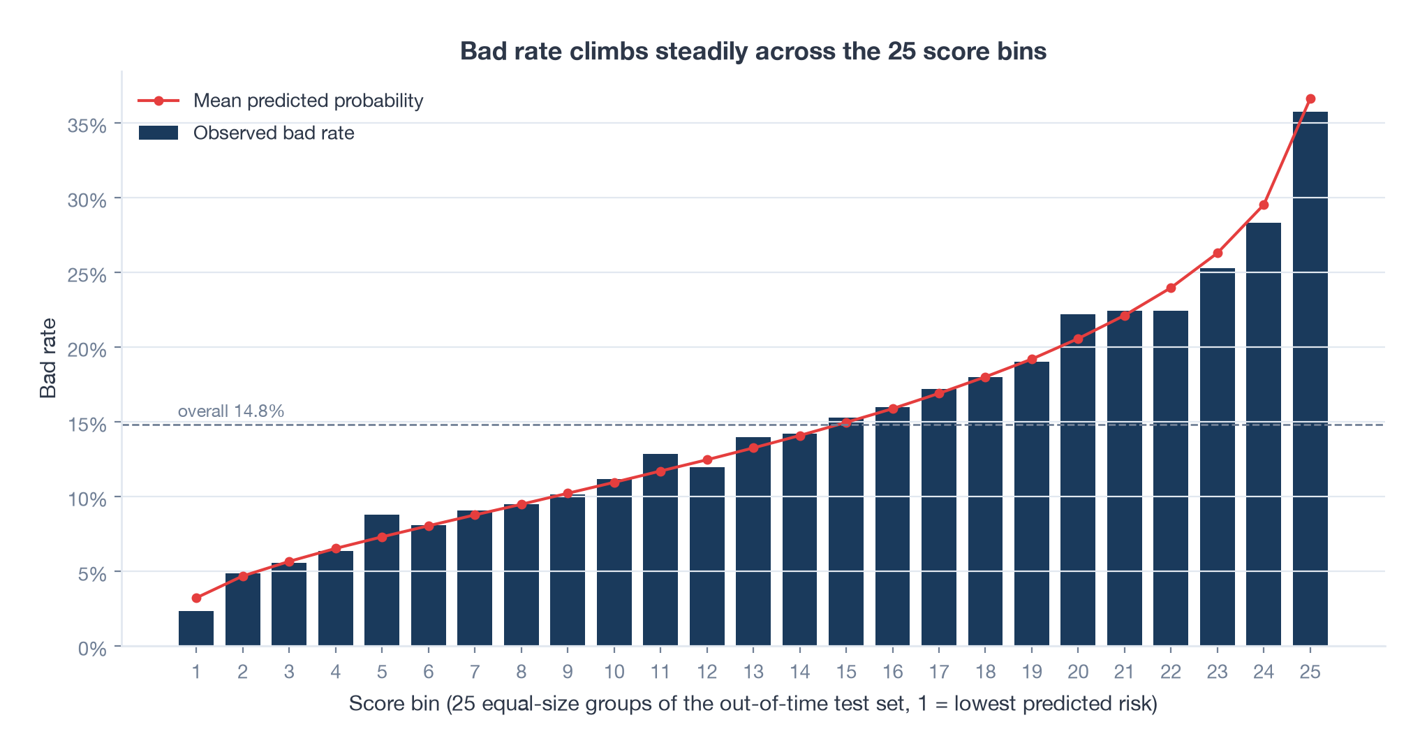
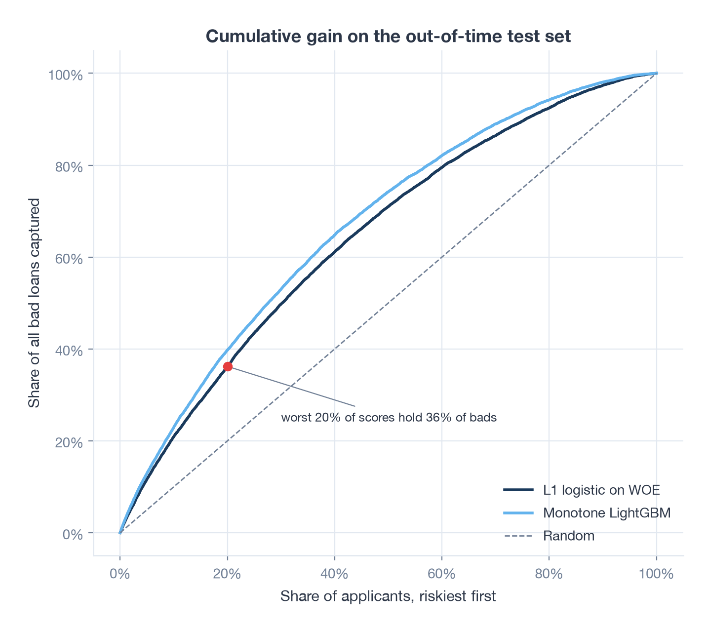
The bad rate climbs from 2.3% in the best bin to 35.8% in the worst, about 15 to 1, and the predicted line sits on top of the observed bars, which means the model is calibrated as well as ranked. The riskiest 20% of scores hold 36% of all defaults for the scorecard and 40% for the LightGBM challenger.
Scaling to a score
In 2018 I mapped probabilities onto 100 to 1000 with a linear transform of log(p), which is not the log-odds, and wrote that twice the risk cost 165 points. Neither claim survives. The industry convention is points to double the odds (PDO): pick a base score, the odds it stands for, and how many points double those odds, and the whole scorecard follows.
import numpy as np

BASE, BASE_ODDS, PDO = 600, 50, 20                 # 600 points at 50:1 good:bad odds
factor = PDO / np.log(2)                           # 28.85 points per unit of log-odds
offset = BASE - factor * np.log(BASE_ODDS)         # 487.1

score = offset + factor * np.log(p_good / p_bad)

# points per bin, so the scorecard can be printed as a table
points = -factor * (coef[feature] * woe_of_bin + intercept / n_features) + offset / n_features
The second formula spreads the intercept evenly over the features so each bin’s points can be read and added up by hand. Here is the debt-to-income row of the card:
| DTI bin | Loans in training | Bad rate | WOE | Points |
|---|---|---|---|---|
| under 7.7 | 20,656 | 11.1% | 0.34 | 32 |
| 7.7 to 12.6 | 33,183 | 11.7% | 0.28 | 31 |
| 12.6 to 15.5 | 23,462 | 13.1% | 0.15 | 28 |
| 17.1 to 21.0 | 31,154 | 14.6% | 0.03 | 26 |
| 25.5 to 27.4 | 10,287 | 18.1% | -0.23 | 21 |
| 33.7 and over | 9,812 | 22.4% | -0.50 | 16 |
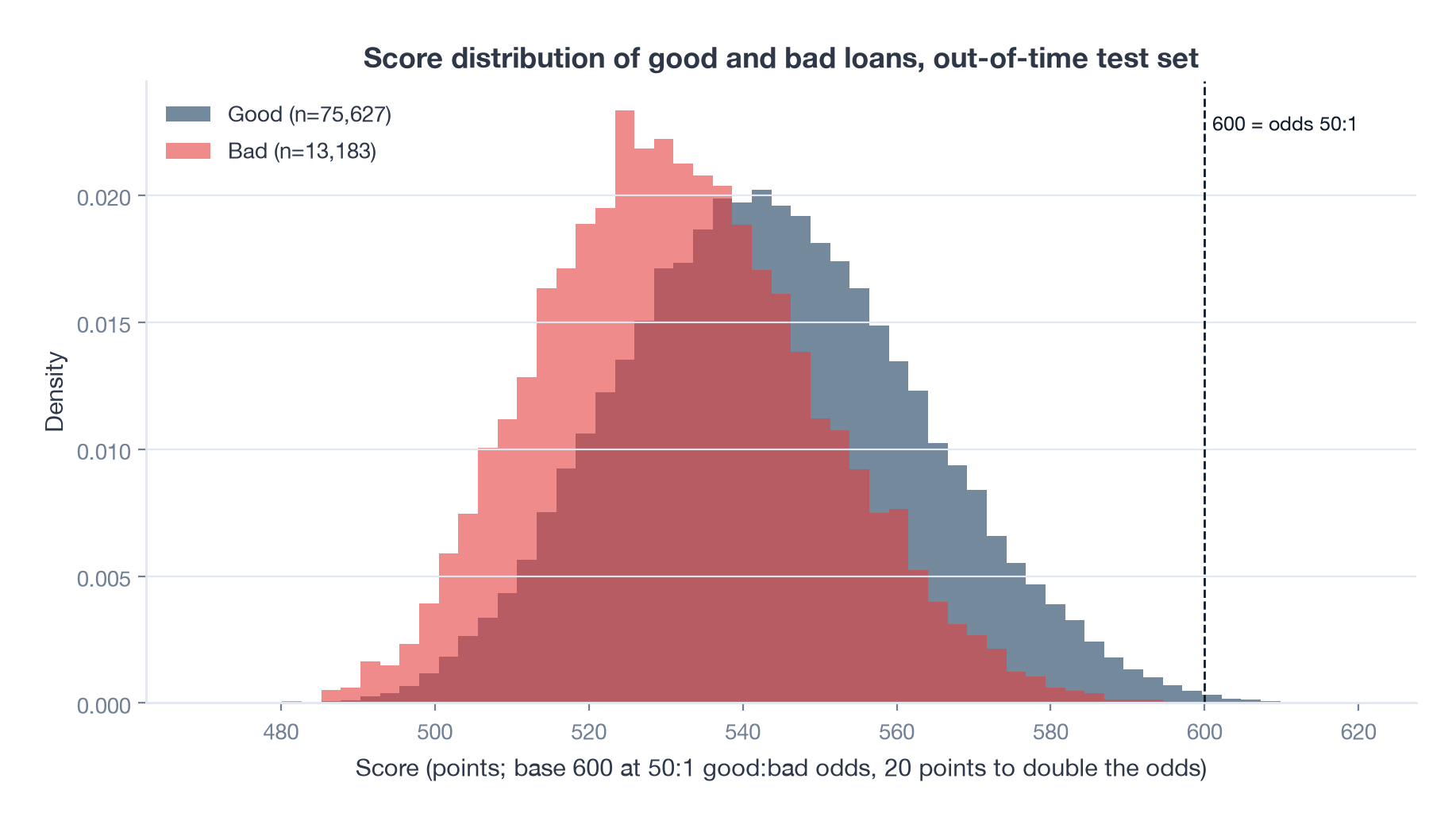
Scores on the test set run from 478 to 616, with a median of 543 for good loans and 531 for bad ones. By band, the bad rate falls from 40% below 500 to 2.9% between 575 and 600. Almost nothing scores above 600, because 600 stands for 50 to 1 odds, a 2% default rate, and this is a 15% book. The base point is a convention, not a cutoff, and a lender would set the approval line wherever the bad rate meets its risk appetite.
What changed between 2018 and 2026
| 2018, R | 2026, Python | |
|---|---|---|
| Feature screen | By hand; a few post-origination columns slipped through | Explicit exclusion list with reasons; application-time only |
| Binning | Information, 10 equal-frequency bins, fitted before the split | optbinning, monotonic bins, fitted on the training window |
| Test | Random 25% | Out of time, last quarter of the year |
| Reported AUC | 0.88 | 0.67 |
| Coefficient signs | Not checked | Five wrong-sign features dropped |
| Challenger | None | Monotone LightGBM, AUC 0.70, explained with SHAP |
| Reject inference | Bugged; no real rejects | Parcelling on 300,000 real 2015 rejects, judged on real outcomes only |
| Grades | 25 equal-width bins | 25 equal-frequency bins, calibration checked |
| Score | Linear in log(p), 100 to 1000 | Points to double the odds, printable points table |
Looking back from 2026
The method held up and the result did not, and I would rather have it that way round. Weight of Evidence and Information Value are still how a scorecard gets built, because they produce a model a regulator can read. What I lacked in 2018 was the discipline around the model: a written list of what a feature is allowed to be, a test set from the future, and a sign check on every coefficient. None of that is hard. All of it changes the answer.
The 0.88 that I published was leakage, and the only reason I can say so with confidence is that the re-run is on the same loan book with the same labels. If you have an old model with a number that looks too good, that is the check: rebuild it with the feature list written down and the test set drawn from after the training window, and see what survives.
The boosted challenger is now part of the routine rather than a nice-to-have. It tells you how much the scorecard leaves behind (here, 0.03 of AUC) and, through SHAP, which interactions it is missing. Lenders increasingly ship the constrained boosted model itself, with adverse-action reasons generated from SHAP, and the explainability bar has risen to meet it. The fairness review has risen too: dropping zip code is the floor, and a production model would be tested for disparate impact across protected groups whether or not those groups are in the data.
Reject inference remains the step I trust least. With real rejects and a careful method it still made the model worse on real outcomes, because the rejects file was recorded with less care than the loans file. The right fix is operational, not statistical: approve a small random slice of marginal rejects and watch what happens to them, so the next scorecard has real outcomes where this one had a factor of two.